library(tidyverse)  # contains ggplot2 and other stuff for data wrangling
library(sf)
library(bruneimap)
postdir <- "posts/brunei-rivers/"
here::i_am(paste0(postdir, "index.qmd")) # Working directoryIt is the 11th day of Ramadhan–a time filled with both reflection and quiet productivity. During this blessed month I have the opportunity to rise and a little earlier than usual. Once my morning tasks were complete, I settled in front of my computer, ready to dive into work.
A particularly intriguing message awaited my attention. Feezul had sent over a an exquisitely detailed image of the rivers of Brunei. The illustration was precise enough that it allowed one to distinguish the subtle curves of the estuaries from the meandering tributaries. (Note to self: I have not used these terms, estuaries and tributaries, in years!) For some inexplicable reason, the image whisked me back to my school days–a time when I and other schoolchildren eagerly memorised the names of Brunei’s four major rivers (a breeze, given that they’re named after their respective districts!). Yet, as the image so delightfully reveals, there’s a far richer tapestry than just these four waterways.
The accompanying LinkedIn post not only credits the data source but also offers an easy tutorial using QGIS—so straightforward that the entire process can be wrapped up in just 10-15 minutes.
Then a curious thought struck: how long would it take to recreate this visual masterpiece using R? Without a moment’s hesitation, I quipped (quietly, since my daughter was still asleep) “Hey Siri, set a timer for 15 minutes”. I fired up RStudio and started coding.
The first step was to load the necessary libraries. For this, I am relying on the {sf} package to handle the spatial data and {ggplot2} for the plotting. The {bruneimap} package also comes in handy here, which contains polygon objects of Brunei. Check out the package here.
Next, we need to get the data. Thanks to the LinkedIn post, I had a direct link to the data source provided by HydroSHEDS. As the website says, the HydroRIVERS v1.0 data set is freely available for scientific, educational, and commercial use. A quick look at the technical documentation confirmed that the Australasia data set in Shapefile format was exactly what I needed.
# Download the data (46.4 MB)
if (!file.exists(here::here(postdir, "HydroRIVERS_v10_au_shp/HydroRIVERS_v10_au.shp"))) {
  download.file(
    url = "https://data.hydrosheds.org/file/HydroRIVERS/HydroRIVERS_v10_au_shp.zip",
    destfile = here::here(postdir, "HydroRIVERS_v10_au_shp.zip")
  )
  unzip(
    zipfile = here::here(postdir, "HydroRIVERS_v10_au_shp.zip"),
    exdir = here::here(postdir)
  )
}
Loading libraries to data acquisition took just three minutes. So far, so good. Next, it’s time to load the data into R.
rivers_sf <- sf::read_sf(here::here(postdir, "/HydroRIVERS_v10_au_shp/HydroRIVERS_v10_au.shp"))
glimpse(rivers_sf)
Rows: 836,472
Columns: 15
$ HYRIV_ID <int> 50000001, 50000002, 50000003, 50000004, 50000005, 50000006,…
$ NEXT_DOWN <int> 50000003, 50000003, 0, 0, 0, 0, 0, 0, 0, 0, 0, 0, 0, 500000…
$ MAIN_RIV <int> 50000003, 50000003, 50000003, 50000004, 50000005, 50000006,…
$ LENGTH_KM <dbl> 1.59, 5.04, 1.07, 1.28, 2.68, 1.33, 1.76, 1.09, 0.69, 0.69,…
$ DIST_DN_KM <dbl> 1.5, 1.3, 0.0, 0.0, 0.0, 0.0, 0.0, 0.0, 0.0, 0.0, 0.0, 0.0,…
$ DIST_UP_KM <dbl> 3.0, 7.9, 9.0, 3.5, 4.5, 2.9, 3.6, 2.4, 2.0, 2.5, 2.8, 3.2,…
$ CATCH_SKM <dbl> 3.61, 16.66, 2.21, 4.01, 7.63, 3.41, 4.63, 2.62, 3.22, 3.42…
$ UPLAND_SKM <dbl> 3.6, 16.7, 22.1, 3.6, 7.4, 3.2, 4.0, 2.4, 2.8, 3.2, 2.2, 3.…
$ ENDORHEIC <int> 0, 0, 0, 0, 0, 0, 0, 0, 0, 0, 0, 0, 0, 0, 0, 0, 0, 0, 0, 0,…
$ DIS_AV_CMS <dbl> 0.153, 0.678, 0.895, 0.153, 0.312, 0.136, 0.198, 0.120, 0.1…
$ ORD_STRA <int> 1, 1, 2, 1, 1, 1, 1, 1, 1, 1, 1, 1, 2, 1, 1, 1, 1, 1, 1, 2,…
$ ORD_CLAS <int> 2, 1, 1, 1, 1, 1, 1, 1, 1, 1, 1, 1, 1, 2, 1, 1, 1, 1, 1, 1,…
$ ORD_FLOW <int> 7, 7, 7, 7, 7, 7, 7, 7, 7, 7, 7, 7, 7, 7, 7, 7, 7, 7, 7, 6,…
$ HYBAS_L12 <dbl> 5120031120, 5120031120, 5120031120, 5120031120, 5120031120,…
$ geometry <LINESTRING [°]> LINESTRING (121.8375 20.75,..., LINESTRING (121.…As per the technical document, this dataset should contain LINESTRING objects representing rivers across the vast Australasia region. Indeed, there are 836472 such features (rivers). So we’ll need to filter for the rivers in Brunei. My strategy here is to use st_intersection() from the {sf} package, but from experience this takes a bit of time if the data set is huge (which, in this case, it is!). So before doing that, I’ll crop out the rivers that are contained within Brunei’s bounding box, making use of the {bruneimap} package. Here’s how I pieced it together:
bbox <- st_bbox(bruneimap::brn_sf)
bnrivers_sf <-
  st_crop(rivers_sf, bbox) |>
  st_intersection(bruneimap::brn_sf)
Warning: attribute variables are assumed to be spatially constant throughout
all geometries
Warning: attribute variables are assumed to be spatially constant throughout
all geometriesA quick check confirmed I was indeed on the right track:
glimpse(bnrivers_sf)Rows: 1,100
Columns: 16
$ HYRIV_ID <int> 50049203, 50049379, 50049412, 50049413, 50049449, 50049450,…
$ NEXT_DOWN <int> 0, 0, 50049379, 50049412, 50049412, 50049412, 50049379, 0, …
$ MAIN_RIV <int> 50049203, 50049379, 50049379, 50049379, 50049379, 50049379,…
$ LENGTH_KM <dbl> 1.62, 1.12, 1.12, 0.69, 0.46, 1.35, 1.96, 2.56, 1.35, 1.61,…
$ DIST_DN_KM <dbl> 0.0, 0.0, 1.4, 2.4, 2.4, 2.6, 1.4, 0.0, 3.0, 5.0, 3.4, 2.8,…
$ DIST_UP_KM <dbl> 3.2, 10.3, 5.7, 2.7, 4.7, 2.5, 9.2, 4.0, 2.3, 3.3, 4.9, 4.3…
$ CATCH_SKM <dbl> 2.99, 1.28, 1.28, 2.57, 0.64, 2.78, 3.21, 9.62, 3.21, 4.28,…
$ UPLAND_SKM <dbl> 2.8, 47.7, 13.7, 2.6, 7.1, 2.8, 33.1, 9.4, 3.2, 4.3, 11.1, …
$ ENDORHEIC <int> 0, 0, 0, 0, 0, 0, 0, 0, 0, 0, 0, 0, 0, 0, 0, 0, 0, 0, 0, 0,…
$ DIS_AV_CMS <dbl> 0.190, 3.263, 0.939, 0.175, 0.485, 0.190, 2.266, 0.646, 0.2…
$ ORD_STRA <int> 1, 3, 2, 1, 2, 1, 3, 1, 1, 1, 2, 1, 1, 2, 1, 2, 1, 2, 1, 1,…
$ ORD_CLAS <int> 1, 1, 2, 4, 2, 3, 1, 1, 3, 2, 2, 2, 3, 1, 2, 1, 2, 1, 2, 5,…
$ ORD_FLOW <int> 7, 6, 7, 7, 7, 7, 6, 7, 7, 7, 7, 7, 7, 6, 7, 7, 7, 7, 7, 7,…
$ HYBAS_L12 <dbl> 5120018310, 5120018310, 5120018310, 5120018310, 5120018310,…
$ name <chr> "Mainland", "Mainland", "Mainland", "Mainland", "Mainland",…
$ geometry <LINESTRING [°]> LINESTRING (115.0521 5.0291..., LINESTRING (114.…ggplot(bnrivers_sf) + geom_sf()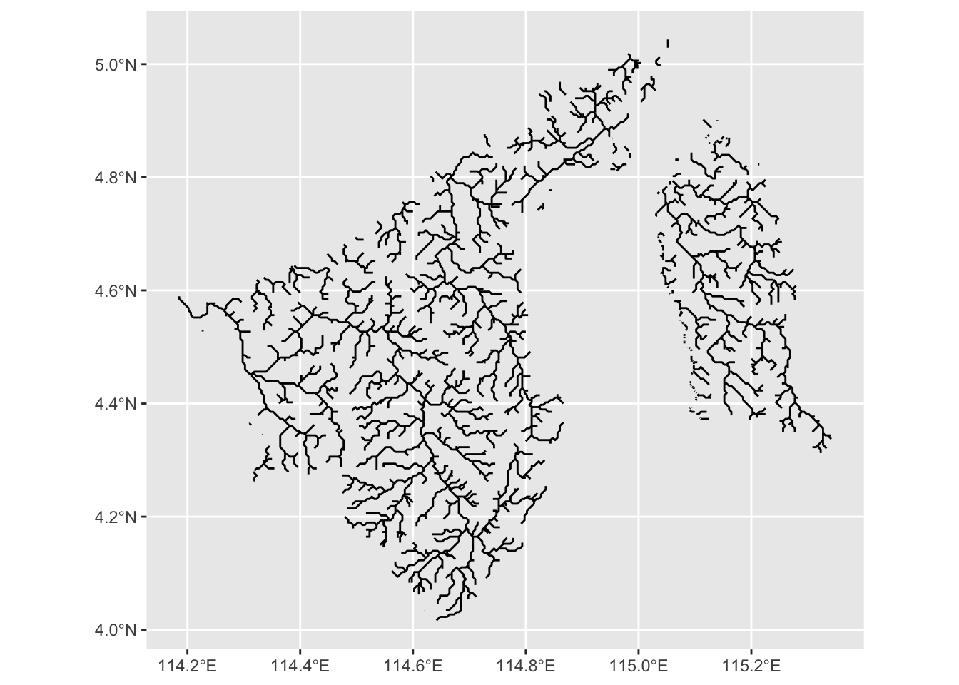
All I have to do now is prettify the plot. From the original image, I observed that the major rivers appeared ever so slightly chunkier than the minor ones, and there was a playful interaction of transparency. I needed to decide which variable in the dataset would best map to the linewidth and alpha aesthetics in my ggplot() call. My first thought was to use the ORD_CLAS variable, which is a measure of river order following the Strahler system. My initial attempt at prettifying the image yielded the following:
bnrivers_sf |>
  filter(ORD_CLAS %in% 1:3) |>  # Only the first three orders
  ggplot() +
  geom_sf(aes(alpha = ORD_CLAS, linewidth = ORD_CLAS)) +
  scale_alpha_continuous(range = c(1, 0.5)) +
  scale_linewidth_continuous(range = c(0.8, 0.5)) +
  theme_void() +
  theme(legend.position = "none")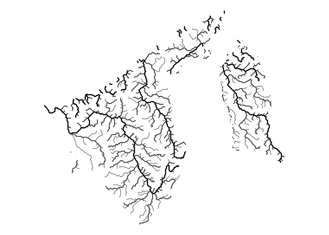
The result looked… adequate, but not quite striking. Twelve minutes had already flown by. I could have stopped there, but I wanted to elevate the visualization further. After all, people count on me to present a compelling use case for R! (Do they, though?) The thing is, I felt that I needed to really study the variables in the data set to figure out which one would be suitable to use for the aesthetics. That could take a while. I know almost nothing about rivers, so I decided to ask good ’ol ChatGPT for guidance.
I prompted ChatGPT to suggest which of the variables in the data set would be suitable for mapping to the aesthetics, even giving it the codebook so it can help me out better. And this is what it come back with:
bnrivers_sf |>
  mutate(log_dis = log(DIS_AV_CMS + 1)) |>
  filter(DIS_AV_CMS > 0.1) |>
  ggplot() +
  geom_sf(aes(linewidth = log_dis, alpha = log_dis), color = "white") +
  scale_linewidth_continuous(range = c(0.3, 1.1)) +
  scale_alpha_continuous(range = c(0.2, 1)) +
  labs(
    title = " The Rivers of Brunei Darussalam",
    subtitle = " Major rivers highlighted by average discharge",
    caption = "Data Source: HydroSHEDS \nCreated by: Haziq J "
  ) +
  theme_void() +
  theme(
    legend.position = "none",
    panel.background = element_rect(fill = "#0e1111", color = "#0e1111"),
    plot.background  = element_rect(fill = "#0e1111", color = "#0e1111"),
    plot.title       = element_text(color = "#FBFAF5", size = 20, face = "bold"),
    plot.subtitle    = element_text(color = "#FBFAF5", size = 14),
    plot.caption     = element_text(color = "#FBFAF5", size = 10)
  )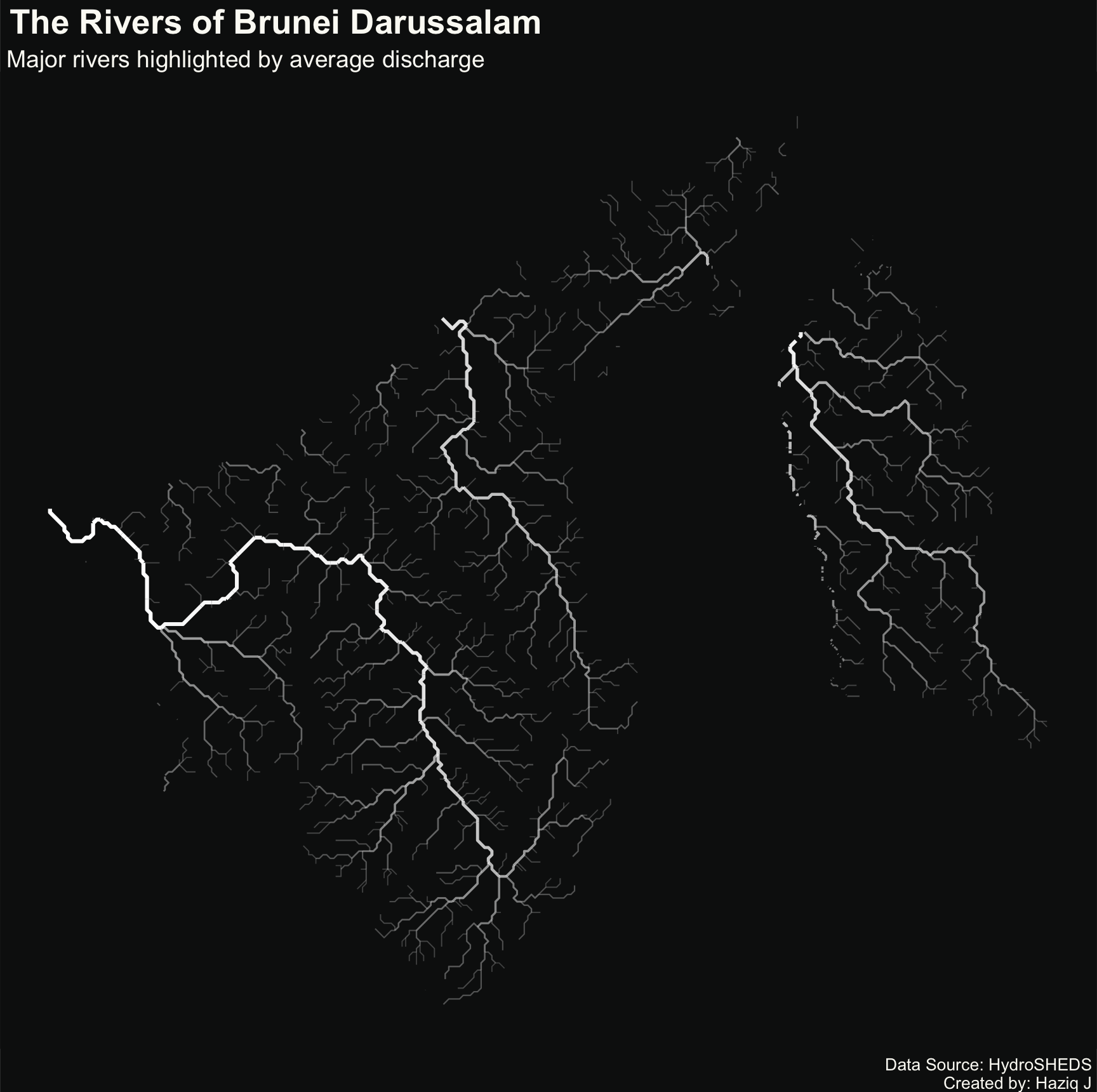
With a bit of fine-tuning on my part, the final visualisation bore an uncanny resemblance to the polished outputs of QGIS. Just as I was wrapping up, the timer went off. It was time to head to campus for a teaching day. What a fun way to start the day!